
Target probability profiles use the uncertainty surrounding your estimation inputs (productivity, labor rate, and size) to generate a sampling distribution of likely effort, cost, quality, and schedule outcomes. The width of this distribution is driven by the uncertainty surrounding your estimation inputs.
Input uncertainty is set by adjusting the uncertainty
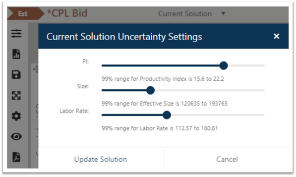
sliders in the flyout menu section of the Contingency dashboard. As you move the
uncertainty sliders from left (lower uncertainty) to right (higher uncertainty),
a 99% confidence range for each metric value is calculated and displayed in the
hover tips for each slider. This range is used during Monte Carlo
simulation to vary each input within its associated uncertainty range and
calculate the full range of potential solutions on probability charts and
reports.
![]()
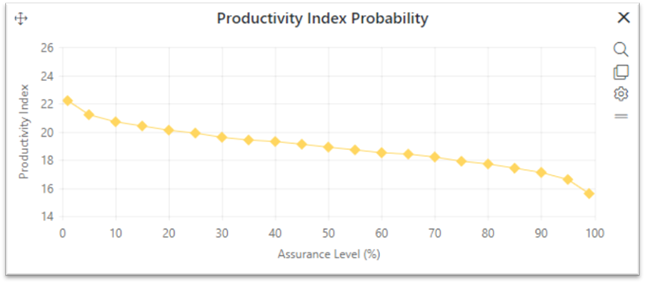
More input uncertainty produces a wider range of potential outcomes; less uncertainty narrows the range of possible outcomes. The probability chart below shows the range within which PI is varied (15.6-22.2) when the PI uncertainty slider is adjusted as shown in the screen snap above.
Once SLIM-Collaborate has generated a distribution of
potential outcomes, estimators can display and compare saved target probability
profiles on Contingency Dashboard charts and reports. Examples might
include:
•65% assurance on time and effort. Provides minimal contingency (buffer).
•95% assurance on time and effort. Provides generous contingency (buffer).
It’s important to understand that the current/50%
probability (or expected) solution is based on the values you provided for your
estimation inputs. Consequently, it does not change as input uncertainties are
adjusted. Adjusting input uncertainty affects only the amount of
risk buffer needed to provide higher assurance (more risk buffer). Thus, a
95% assurance contingency solution will be different if uncertainty is low than
when uncertainty is high. The amount of risk buffer scales with the amount
of uncertainty surrounding the solution inputs.
In the charts below, the yellow curves represent the
current solution (the expected outcome based on your best estimates for inputs
like productivity and final system size). The grey time series curves show
the 65% assurance and 95% assurance, risk buffered solutions. These
“contingency” solutions help estimators visualize and assess the amount of
additional contingency needed to allow firms to negotiate commitments that
contain a reasonable amount of management reserve.

For more detailed guidance on working with target
probability profiles, see the Creating
Target Probability Solutions and Creating a Contingency Profile
sections of this user guide.