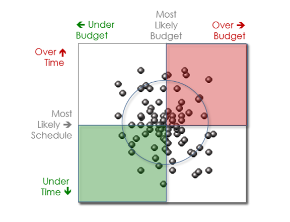
When you adjust the uncertainty sliders, SLIM-Collaborate will run a Monte Carlo simulation to update the range of solutions shown on probability charts and reports in the Contingency dashboard.
During the Monte Carlo simulation, the size, PI, labor rate, and MBI are varied randomly about their expected values within statistical limits set by their respective standard deviations. One hundred solutions are calculated by selecting solution parameters from a normal distribution around the average or expected value. Some of these solutions will exceed the expected schedule, budget, and staffing and some will come in lower than the planned values. Most solutions, however, will cluster somewhere in the middle.

You can think of these solutions as “what if” estimates –
“What if the size is only half what we estimated?”, or “What if the size
doubles?”. Or in the case of productivity, “What if we are more or less
productive than we expected to be?”. Varying the inputs allows
SLIM-Collaborate to translate uncertainty surrounding inputs like size or PI to
uncertainty on the outputs for the estimate: effort, cost, schedule, and
size.
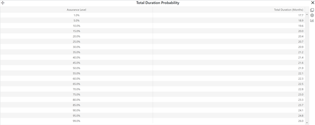
Once Monte Carlo simulation is complete, probability distributions are generated for the major management metrics and displayed on Probability charts and reports. The example below shows the range of schedule outcomes associated with a current Estimation service solution.
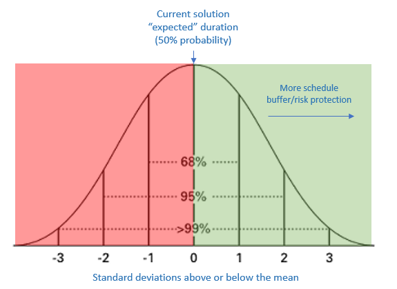
Note that the current – or “expected” - solution is always at the center (50% assurance level) of this cumulative distribution. Solutions with a higher than 50% assurance have some schedule contingency built in. If you want to be 90% certain of not exceeding your planned (expected) schedule of 21.9 months, you will need about 2.2 months of schedule buffer (24.1 months).

NOTE: Fixed percentage contingency profiles allow estimators to apply a fixed amount of risk buffer (for example, 10% on schedule and 30% on effort or cost) to an existing estimate. They are independent of input uncertainty.